Image 1. IBM Power Systems

Introduction

Image classification has become one of the key pilot cases for demonstrating machine learning. In the previous article, I introduced machine learning, IBM PowerAI, compared GPU and CPU performances while running image classification programs on the IBM Power platform. In this article, let’s take a look at how to check the output at any inner layer of a neural network and train your own model by working with Nvidia DIGITS.

Observing hidden layer parameters

It wasn’t till the 1980s that researchers discovered adding more layers to a neural network vastly improved its performance. Such neural networks with several hidden layers are common today in several use cases including image classification. Contrary to what the name indicates, it is possible to observe relevant parameters in the hidden layers.

Convolutional Neural Network Architecture

As you probably know by now, convolutional neural networks (CNNs) are a type of deep neural network and produce fairly accurate results when used for image classification.

When studying Digital Signal Processing in engineering school, you are bound to come across the term convolution. Simply put, the convolution of two signals is the integration of the product of the two signal functions, after one of the functions is reversed and shifted. In our case, every input image is a matrix of pixel values. To see a visual representation of how convolution is performed in the hidden layers, consider this example.

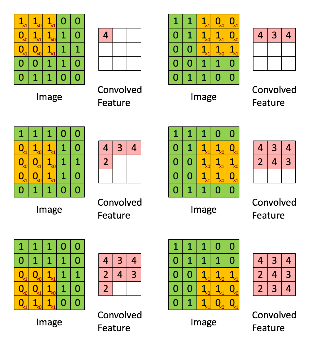Image 2. Convolution, Source

In this example, the orange matrix (3x3) is called the Filter and is used to compute a convoluted output of the original image (5X5 matrix of pixels). The result is called the Activation Map or Feature Map. It is to be understood that depending on the Filter applied, the output Feature Map can be modified and trained to get the desired output.

In modern CNNs, the Filter is learned automatically during the training process, but we do specify certain parameters (shown below) depending on the architecture being used. Please head to this blog if you need a more detailed analysis.

In our case, a version of AlexNet is used and that’s the standard architecture we rely on. In the code below, we read the structure of the net. The CNN contains two ordered dictionaries;

1. **Net.blobs** for input data;

a. This has the following parameters – batch size, channel dimension, height and width

2. **Net.params** is a vector of blobs for having weight and bias parameters;

a. Weight indicates the strength of a connection. Weights near zero indicate a good correlation between the input and the ouput.

b. Bias indicates how far off the predictions may be from the real values and is very important in moving the predictions along to the next step.

c. This has the following parameters – output channels, input channels, filter height and filter width for the weights and a one-dimentional output channel for the biases.

Let’s attempt to print these.

\# for each layer, show the output shape
for layer\_name, blob in net.blobs.iteritems():
print layer\_name + ‘\\t’ + str(blob.data.shape)

Here is the output.

data (50, 3, 227, 227)
conv1 (50, 96, 55, 55)
pool1 (50, 96, 27, 27)
norm1 (50, 96, 27, 27)
conv2 (50, 256, 27, 27)
pool2 (50, 256, 13, 13)
norm2 (50, 256, 13, 13)
conv3 (50, 384, 13, 13)
conv4 (50, 384, 13, 13)
conv5 (50, 256, 13, 13)
pool5 (50, 256, 6, 6)
fc6 (50, 4096)
fc7 (50, 4096)
fc8 (50, 1000)prob (50, 1000)

And;

for layer\_name, param in net.params.iteritems():
print layer\_name + ‘\\t’ + str(param\[0\].data.shape), str(param\[1\].data.shape)

Here is the output.

conv1 (96, 3, 11, 11) (96,)
conv2 (256, 48, 5, 5) (256,)
conv3 (384, 256, 3, 3) (384,)
conv4 (384, 192, 3, 3) (384,)
conv5 (256, 192, 3, 3) (256,)
fc6 (4096, 9216) (4096,)
fc7 (4096, 4096) (4096,)
fc8 (1000, 4096) (1000,)

As you see, we have four dimensional data here. Here is a function to visualize this data;

def vis\_square(data):  
“””Take an array of shape (n, height, width) or (n, height, width, 3)  
 and visualize each (height, width) thing in a grid of size approx. sqrt(n) by sqrt(n)”””  
   
 # normalize data for display  
 data = (data — data.min()) / (data.max() — data.min())  
   
 # force the number of filters to be square  
 n = int(np.ceil(np.sqrt(data.shape\[0\])))  
 padding = (((0, n \*\* 2 — data.shape\[0\]),  
 (0, 1), (0, 1)) # add some space between filters  
 + ((0, 0),) \* (data.ndim — 3)) # don’t pad the last dimension (if there is one)  
 data = np.pad(data, padding, mode=’constant’, constant\_values=1) # pad with ones (white)  
   
 # tile the filters into an image  
 data = data.reshape((n, n) + data.shape\[1:\]).transpose((0, 2, 1, 3) + tuple(range(4, data.ndim + 1)))  
 data = data.reshape((n \* data.shape\[1\], n \* data.shape\[3\]) +  data.shape\[4:\])  
   
 plt.imshow(data); plt.axis(‘off’)

Here, you can see the filters in the layer conv1;

\# the parameters are a list of \[weights, biases\]
filters = net.params\[‘conv1’\]\[0\].data
vis\_square(filters.transpose(0, 2, 3, 1))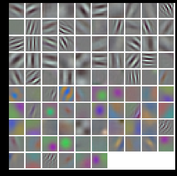

Image 3. Filters in a layer

Here, we see rectified responses of the filters above for the first 36;

feat = net.blobs\[‘conv1’\].data\[0, :36\]
vis\_square(feat)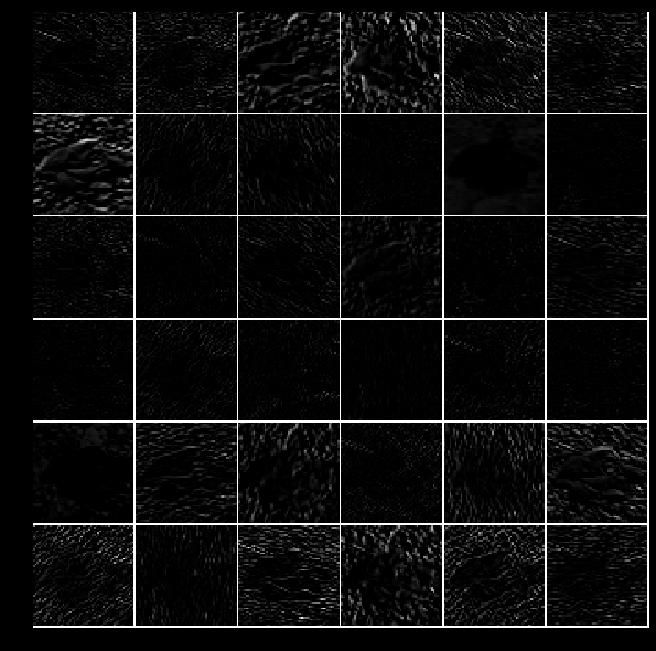

Image 4. Rectified output

Here, we see the output of the fifth layer, after pooling has been done;

feat = net.blobs\[‘pool5’\].data\[0\]
vis\_square(feat)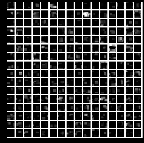

Image 5. Output of the fifth layer after pooling

The first fully connected layer was ‘fc6’ which is a rectified output. The histogram of all non-negative values is displayed using this code;

feat = net.blobs\[‘fc6’\].data\[0\]
plt.subplot(2, 1, 1)
plt.plot(feat.flat)
plt.subplot(2, 1, 2)\
_ = plt.hist(feat.flat\[feat.flat > 0\], bins=100)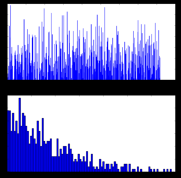

Image 6. Histogram of rectified output — More explanation in this blog

Here, we see the histogram of the final probability values of all predicted classes. The top peak here shows the top predicted class, in our case, orangutan. Other minor cluster peaks are also shown.

feat = net.blobs\[‘prob’\].data\[0\]
plt.figure(figsize=(15, 3))
plt.plot(feat.flat)\
[<matplotlib.lines.Line2D at 0x7f09587dfb50>\]

Image 7. The top peak here shows the top predicted class, in our case, orangutan

How to train your own machine learning model?

What is Nvidia DIGITS?

Nvidia Deep Learning GPU Training System (DIGITS) is an application that is used to classify images, perform segmentation and object detection tasks. It is a GUI based application that interfaces with Caffe. The download and installation procedure can be found on their website. Stable and other beta versions are also available on Github. DIGITS server is installed in the container that I am using for this demo. Once installed, the GUI can be accessed from port 5000.

The next step is to download a sample dataset from the web to a directory I created (/DIGITS) in my VM. This dataset is called CIFAR-100. It contains 100 classes of images and each class contains 600 images. There are 500 training images and 100 testing images per class. The 100 classes in the CIFAR-100 are grouped into 20 super-classes. Each image comes with a “fine” label (the class to which it belongs) and a “coarse” label (the super-class to which it belongs).

Here’s a brief explanation of what it contains;

1. Labels.txt: This file contains a list of classes in the training data set.

2. Train: This directory contains the images used for training.

3. Train.txt: This file contains a list of mappings between training files to the classes. The labels are positional, i.e. the first label from the labels.txt file is represented by the number 0, the second by number 1 etc.

4. Test: This directory contains the images used for testing the training quality.

5. Test.txt: This file contains a list of mappings between the test files and the classes. The labels are positional, i.e. the first label from the labels.txt file is represented by the number 0, the second by number 1 etc.

root@JARVICENAE-0A0A1841:~/DIGITS# python -m digits.download\_data cifar100 .

The output;

Downloading url=http://www.cs.toronto.edu/~kriz/cifar-100-python.tar.gz …
Uncompressing file=cifar-100-python.tar.gz …
Extracting images file=./cifar-100-python/train …
Extracting images file=./cifar-100-python/test …
Dataset directory is created successfully at ‘.’
Done after 65.3251469135 seconds.

Let’s take a look at the downloaded data set. Although I am not showing the other directories I listed above, assume that they are downloaded and present.

root@JARVICENAE-0A0A1841:~/DIGITS# ls fine/train | head
apple
aquarium_fish
baby
bear
beaver
bed
bee
beetle
bicycle
bottle

Let’s create a new classification dataset with the pre-trained dataset (CIFAR-100) that we downloaded.

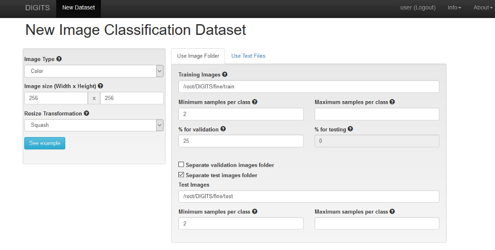Image 8. New Image Classification Dataset on DIGITS

Here, the path /root/DIGITS/fine/train is the path to our dataset. Also notice the ‘Separate test images folder’ option and specify the /root/DIGITS/fine/test directory. You can also specify a name for this dataset, like ‘Cifar100’ for example (not shown in the screenshot above).

When you click on Create, a new job to create the training database is started as shown below.

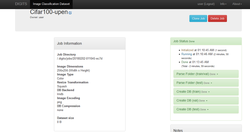Image 9. Job status

The status of the jobs involved are shown on the right hand side pane in the image above. Once done, your DIGITS home screen should now show this dataset as being available to use.

Creating a new image classification model

Let’s create a new image classification model with the name ‘Classify Images’ with the CIFAR-100 dataset we created. We’ll use a pre-built AlexNet neural network architecture for this model.

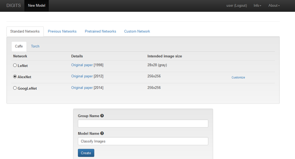Image 10. Job status of new image classification model

Once you click on Create, a new job is started as before. The status of the job called ‘Train Caffe Model’ is shown in the screenshot below.

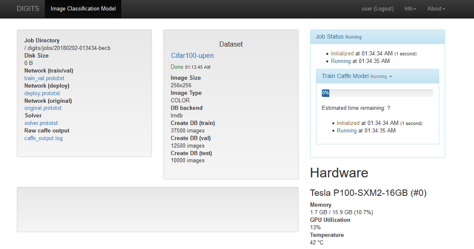Image 11. Training your model

As the training proceeds, the job status will be updated in a graph as shown below. Over time, I was able to see an increase in accuracy.

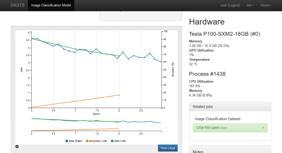Image 12. Sample image classification

After a while, when the job completes, you will be able to upload a test image and classify it based on your model. An example image (of a green apple) is being uploaded and the results are seen instantly.

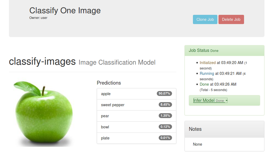Image 13. Sample image classification

This is fairly good accuracy with a small dataset like CIFAR-100, and you can expect better accuracy values when larger datasets are used.

I wish to write a shorter part 3 to show the benefits of Torch. Time will tell.

The postings on this site are my own and don’t necessarily represent IBM’s positions, strategies or opinions.