 Image 1. IBM Power Systems
Introduction
Image classification has become one of the key pilot use cases for demonstrating machine learning. In this short article, I attempt to write about how to implement such a solution using IBM PowerAI, and compare GPU and CPU performances while running this on IBM Power Systems.
Artificial Intelligence
Artificial Intelligence is currently seen as a branch of computer science that deals with making computers perform tasks like visual recognition, speech identification, cognitive decision-making, language translation etc, which are traditionally attributed to human intelligence.
Machine Learning
Machine Learning, commonly viewed as an application of Artificial Intelligence, deals with giving the systems an ability to learn and improve with experience, without explicitly coding all tasks.
Deep Learning
Deep Learning is a subset of Machine Learning where the systems can learn with labelled training data (supervised) or unlabeled training data (unsupervised). Deep Learning typically uses a hierarchical level of artificial neural networks to carry out a task.
Artificial Neural Networks
Artificial Neural Networks are systems inspired by biological neural networks and can perform certain tasks like image classification with amazing accuracy. For example, for image classification, a set of images of an animal are provided with labeling. This is the training data. The Artificial Neural Network, over a series of steps (or layers), helps the system learn the ability to classify unlabeled images (An image of an Orangutan in the example shown in this article) as belonging to a certain group while coming up with accuracy scores.
There are several applications of deep learning for your business, ranging from cellphone personal assistants to self-driving cars where rapidly changing patterns are used to classify objects in real-time.
What is IBM PowerAI?
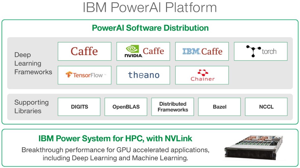
IBM PowerAI software lets you easily run all the popular machine learning frameworks with minimal effort on your IBM POWER9 servers which contain a GPU. CPUs were designed and built for serial processing and contain a small number of cores, whereas GPUs can contain thousands of smaller cores and rely on parallel processing of tasks. Tasks meant for machine learning are key applications of GPUs. Check out the IBM Power System AC922 servers, touted as one of the best servers in the market for running enterprise AI tasks. IBM PowerAI currently includes the following frameworks;
 Image 2. Source: https://www.ibm.com/us-en/marketplace/deep-learning-platform
Current setup
For this demo, I used a container on a VM running Ubuntu on Power ( ppc64le ), hosted on Nimbix Cloud.
A Container is a running instance of an image. An image is a template which contains the OS, Software and application code, all bundled in one file. Images are defined using a Dockerfile, which is a list of steps to configure the image. The Dockerfile is built to create an image, and the image is run to get a running container. To run the image, you need to have Docker Engine installed and configured on the VM.
Here is the Dockerfile I used, written by Indrajit Poddar. This is taken from this Github page.
This builds an image with Jupyter Notebook, iTorch Kernel (we'll discuss this in the second part) and some base TensorFlow examples.
**TensorFlow ** is an open source, scalable library for Machine Learning applications, and is based on the concept of a data flow graph which can be built and executed. A graph can contain two components, nodes and edges (or tensors). It comes with a Python API, and is easy to assemble a net, assign parameters and run your training models.
The steps below were demonstrated by Indrajit Poddar. He has built a test image on Nimbix Cloud which will run the aforementioned services when deployed, in a few minutes.
The following command is used to verify if the GPU is attached to the container.
root@JARVICENAE-0A0A1841:/usr/lib/nvidia-384# nvidia-smi
Thu Feb 1 23:45:11 2018
+ — — — — — — — — — — — — — — — — — — — — — — — — — — — — — — — — — — — — — — -+
| NVIDIA-SMI 384.111 Driver Version: 384.111 |
| — — — — — — — — — — — — — — — -+ — — — — — — — — — — — + — — — — — — — — — — — +
| GPU Name Persistence-M| Bus-Id Disp.A | Volatile Uncorr. ECC |
| Fan Temp Perf Pwr:Usage/Cap| Memory-Usage | GPU-Util Compute M. |
|===============================+======================+======================|
| 0 Tesla P100-SXM2… Off | 00000003:01:00.0 Off | 0 |
| N/A 40C P0 42W / 300W | 299MiB / 16276MiB | 0% Default |
+ — — — — — — — — — — — — — — — — — — — — — — — — — — — — — — — — — — — — — — -+
| Processes: GPU Memory |
| GPU PID Type Process name Usage |
|=============================================================================|
+ — — — — — — — — — — — — — — — — — — — — — — — — — — — — — — — — — — — — — — -+
I see an Nvidia Tesla P100 GPU attached. The following command shows the installed Jupyter Notebook instances and the associated tokens that will be used for authentication later.
root@JARVICENAE-0A0A1841:/usr/lib/nvidia-384# jupyter notebook list
Currently running servers:
http://0.0.0.0:8889/?token=d0f34d33acc9febe500354a9604462e8af2578f338981ad1 :: /opt/DL/torch
http://0.0.0.0:8888/?token=befd7faf9b806b6918f0618a28341923fb9a1e77d410b669 :: /opt/DL/caffe-ibm
http://0.0.0.0:8890/?token=a9448c725c4ce2af597a61c47dcdb4d1582344d494bd132f :: /opt/DL/tensorflow
root@JARVICENAE-0A0A1841:/usr/lib/nvidia-384#
Starting Image Classification
What is Caffe?
**Caffe ** (Convolutional Architecture for Fast Feature Embedding) was developed at the Berkeley Vision and Learning Center. It is an open source framework for performing tasks like image classification. It supports CUDA , Convolutional Neural Networks, has pre-trained models, and is therefore a good choice for this demo.
We'll use Python to perform all the tasks. The steps below were done via Jupyter Notebook. First, let's set up Python, Numpy, and Matplotlib.
import numpy as np
import matplotlib.pyplot as plt
# display plots in this notebook
%matplotlib inline
# set display defaults
plt.rcParams[‘figure.figsize’] = (10, 10) # large images
plt.rcParams[‘image.interpolation’] = ‘nearest’ # don’t interpolate: show square pixels
plt.rcParams[‘image.cmap’] = ‘gray’ # use grayscale output rather than a (potentially misleading) color heatmap
# Then, we load Caffe. The caffe module needs to be on the Python path;
# we’ll add it here explicitly.
import sys
caffe_root = ‘../’ # this file should be run from {caffe_root}/examples (otherwise change this line)
sys.path.insert(0, caffe_root + ‘python’)
import caffe
What is Caffenet?
**Caffenet ** is a convolutional neural network written to interface with CUDA , with the primary aim of classifying images. Caffenet is a variant of Alexnet. A presentation from 2015 by the creators of Alexnet is here. In the code below, we download a pre-trained model.
import os
if os.path.isfile(caffe_root + ‘models/bvlc_reference_caffenet/bvlc_reference_caffenet.caffemodel’):
print ‘CaffeNet found.’
else:
print ‘Downloading pre-trained CaffeNet model…’
!../scripts/download_model_binary.py ../models/bvlc_reference_caffenet
Here is the output.
CaffeNet found.
Downloading pre-trained CaffeNet model...
…100%, 232 MB, 42746 KB/s, 5 seconds passed
Then, we load Caffe in CPU mode and work with input preprocessing.
caffe.set_mode_cpu()
model_def = caffe_root + ‘models/bvlc_reference_caffenet/deploy.prototxt’
model_weights = caffe_root + ‘models/bvlc_reference_caffenet/bvlc_reference_caffenet.caffemodel’
net = caffe.Net(model_def, # defines the structure of the model
model_weights, # contains the trained weights
caffe.TEST) # use test mode (e.g., don’t perform dropout)
Caffenet’s ‘caffe.io.Transformer’ is used. This is the default transformer used in all examples. It creates a transformed mean value for an image based on the input provided. Caffenet is setup to get input images in the BGR format with values in the range 0 to 255. Transformation to load images with values in the range of 0 to 1 in RGB format, as input needed for Matplotlib, are performed.
# load the mean ImageNet image (as distributed with Caffe) for subtraction
mu = np.load(caffe_root + ‘python/caffe/imagenet/ilsvrc_2012_mean.npy’)
mu = mu.mean(1).mean(1) # average over pixels to obtain the mean (BGR) pixel values
print ‘mean-subtracted values:’, zip(‘BGR’, mu)
# create transformer for the input called ‘data’
transformer = caffe.io.Transformer({‘data’: net.blobs[‘data’].data.shape})
transformer.set_transpose(‘data’, (2,0,1)) # move image channels to outermost dimension
transformer.set_mean(‘data’, mu) # subtract the dataset-mean value in each channel
transformer.set_raw_scale(‘data’, 255) # rescale from [0, 1] to [0, 255]
transformer.set_channel_swap(‘data’, (2,1,0)) # swap channels from RGB to BGR
In other words, computers can now learn to classify an image by first converting the image to an array of RGB values. Then, these values are scanned to look for patterns of values that already match another image in a pre-trained model. While comparing, confidence metrics are generated which show how accurate the classification was.
Here is the output.
mean-subtracted values: \[(‘B’, 104.0069879317889), (‘G’, 116.66876761696767), (‘R’, 122.6789143406786)\]Classification
Here, we set the default size of the images. This can be changed later depending on your input.
net.blobs[‘data’].reshape(
50, # batch size
3, # 3-channel (BGR) images
720, 720) # image size is 720x720
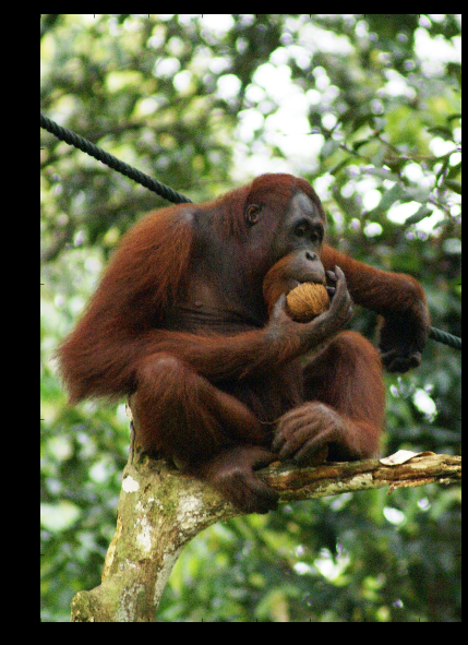
Next, we load the image of an Orangutan from the Wiki Commons library.
# download the image
my_image_url = “https://upload.wikimedia.org/wikipedia/commons/b/be/Orang_Utan%2C_Semenggok_Forest_Reserve%2C_Sarawak%2C_Borneo%2C_Malaysia.JPG" # paste your URL here
!wget -O image.jpg $my_image_url
# transform it and copy it into the net
image = caffe.io.load_image(‘image.jpg’)
transformed_image = transformer.preprocess(‘data’, image)
plt.imshow(image)
Here is the output.
--2018-02-02 00:27:52--  https://upload.wikimedia.org/wikipedia/commons/b/be/Orang_Utan%2C_Semenggok_Forest_Reserve%2C_Sarawak%2C_Borneo%2C_Malaysia.JPG
Resolving upload.wikimedia.org (upload.wikimedia.org)... 198.35.26.112, 2620:0:863:ed1a::2:b
Connecting to upload.wikimedia.org (upload.wikimedia.org)|198.35.26.112|:443... connected.
HTTP request sent, awaiting response... 200 OK
Length: 1443340 (1.4M) [image/jpeg]
Saving to: 'image.jpg'
image.jpg           100%[===================>]   1.38M  5.25MB/s    in 0.3s
2018-02-02 00:27:54 (5.25 MB/s) - 'image.jpg' saved [1443340/1443340]
Image 3. Here's our input image
Now, let’s classify the image.
# copy the image data into the memory allocated for the net
net.blobs[‘data’].data[…] = transformed_image
# perform classification
output = net.forward()
output_prob = output[‘prob’][0] # the output probability vector for the first image in the batch
print ‘predicted class is:’, output_prob.argmax()The output was ‘predicted class is: 365’.
The output above classifies the image into class 365. Let’s load the ImageNet labels and view the output.
# load ImageNet labels
labels_file = caffe_root + ‘data/ilsvrc12/synset_words.txt’
if not os.path.exists(labels_file):
!../data/ilsvrc12/get_ilsvrc_aux.sh
labels = np.loadtxt(labels_file, str, delimiter=’\t’)
print ‘output label:’, labels[output_prob.argmax()]
Here’s the output. The class was correct!
output label: n02480495 orangutan, orang, orangutang, Pongo pygmaeusThe following code helps you come up with other top classes.
# sort top five predictions from softmax output
top_inds = output_prob.argsort()[::-1][:5] # reverse sort and take five largest items
print ‘probabilities and labels:’
zip(output_prob[top_inds], labels[top_inds])
Here is the output.
probabilities and labels:
[(0.96807814, 'n02480495 orangutan, orang, orangutang, Pongo pygmaeus'),
(0.030588957, 'n02492660 howler monkey, howler'),
(0.00085891742, 'n02493509 titi, titi monkey'),
(0.00015429058, 'n02493793 spider monkey, Ateles geoffroyi'),
(7.259626e-05, 'n02488291 langur')]
Analyzing GPU Performance
Here is the time taken to perform the classification on the CPU only mode.
%timeit net.forward()Here is the output.
OUTPUT: 1 loop, best of 3: 3.06 s per loopThree seconds per loop is quite long. Let’s switch to GPU mode and perform the same.
caffe.set_device(0) # if we have multiple GPUs, pick the first one
caffe.set_mode_gpu()
net.forward() # run once before timing to set up memory
%timeit net.forward()
Here is the output.
OUTPUT: 1 loop, best of 3: 11.4 ms per loopThat is an improvement of 3048.6 milliseconds! This concludes the first part of this blog. I apologize for grammatical errors, if any.
In the next part, we will take a look at how to train your own model using NVIDIA Digits and how to use Torch.
Disclaimer: The postings on this site are my own and don’t necessarily represent IBM’s positions, strategies or opinions.